On my commute I listened to a podcast episode featuring Songlin Yang—nicknamed the mother of linear attention—where she patiently explained the mechanics behind the architecture. The structure is red-hot right now, especially because several frontline Chinese model labs are doubling down on it. I figured it was worth retelling the story in my own words.
How Is a Token Generated?
To keep things simple, let’s focus on the inference stage of a large language model—the everyday scenario where a user asks a question. Suppose the prompt is: “I want to see snow over New Year’s. Any destination tips?” Anyone who has used an LLM knows what happens next: the model answers one token at a time.
Every token in that reply can be decomposed into the following stages:
1. Tokenization
We first convert human language into a sequence of numbers; each number is simply an ID. The question above might become something like [37046, 33565, 111, 24186, 6079, 99…]. You’ll notice the sequence length no longer matches the original sentence because the tokenizer may merge or split characters. That detail isn’t crucial for today’s discussion.
2. Embedding
Next comes a giant lookup table. Each token ID corresponds to a long vector that represents the token in a so-called semantic space. Understanding vectors requires some math background, but the intuition is straightforward. Even if “apple” has ID 888 and “banana” has ID 6666—separated by thousands of other tokens like “Silicon Valley” or “large model”—their semantic vectors can still sit close together, while unrelated words stay far apart. We can even do algebra on them.
The classic example is “emperor” - “man” + “woman” ≈ “empress.” That gives a tangible feel for what embeddings do. Once the model is trained, this big table stays fixed.
3. Transformer Processing
The name Transformer often gets associated with the robots-in-disguise franchise, probably because it sounds cool, but the original meaning is closer to an electrical transformer: it converts input into another representation. Modern LLMs stack many Transformer layers—repeating the same principle multiple times.
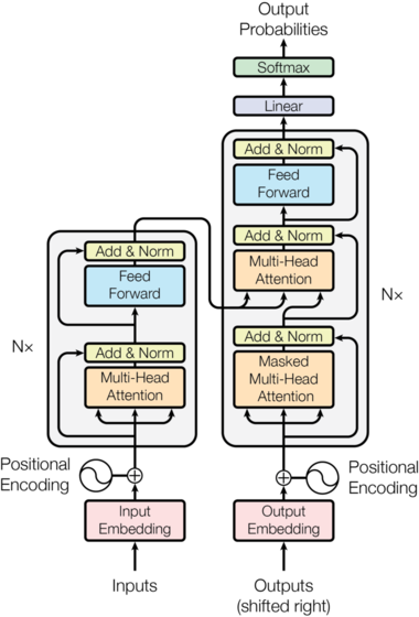
This process revolves around two key steps:
Step One: Self Attention
Self-attention is the celebrity mechanism (and the origin of this newsletter’s name). The idea is intuitive: aggregate the most relevant information from the current context to predict the next token.
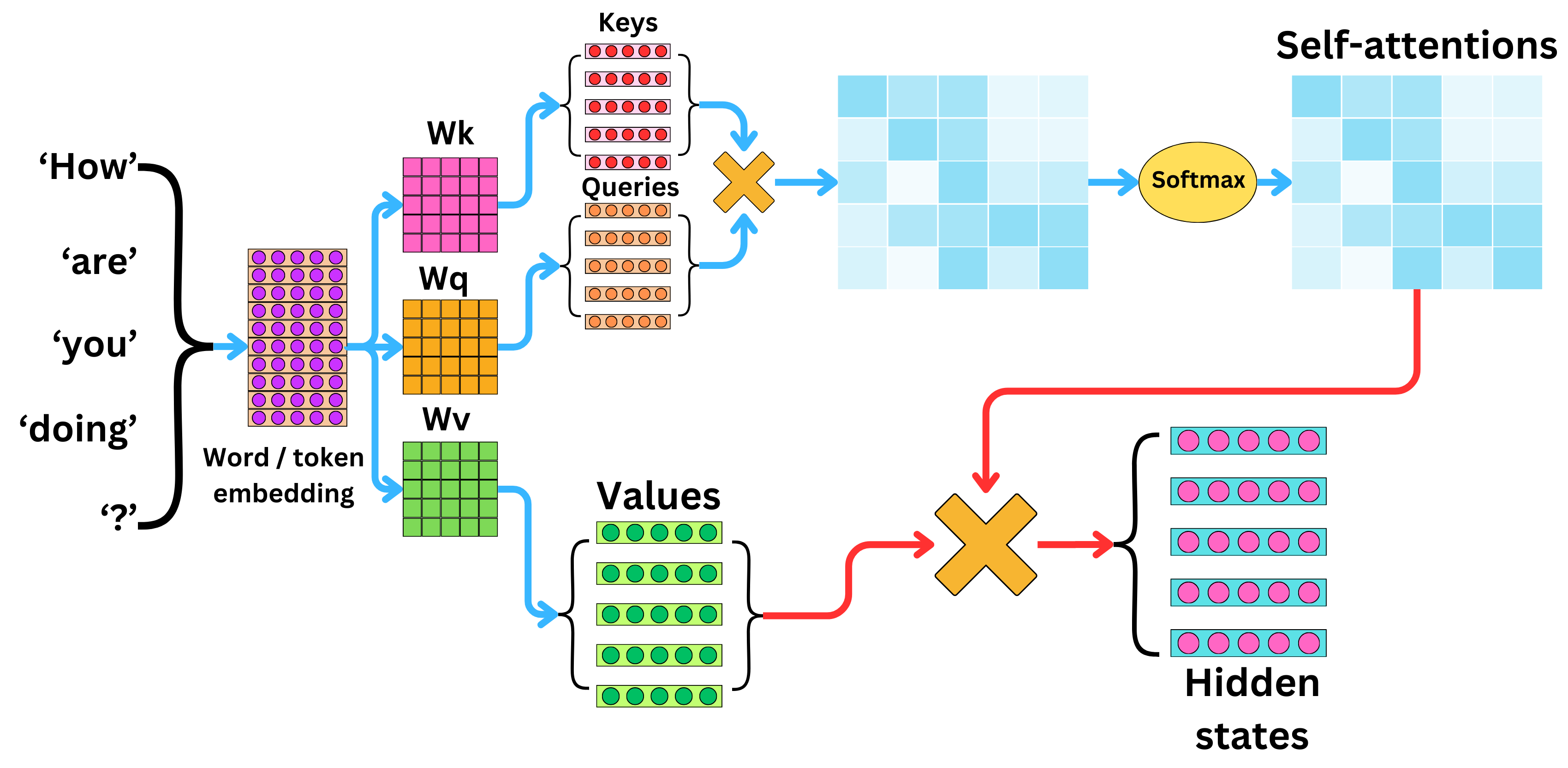
After embedding, we have an $L \times d$ matrix if the context length is $L$ and the embedding dimension is $d$. We project this matrix three ways—multiplying it by three different weight matrices—to obtain $\mathbf{Q}$ (queries), $\mathbf{K}$ (keys), and $\mathbf{V}$ (values).
Take the last query vector $\mathbf{q}_{L}$ and compute its similarity with every key $\mathbf{k}_{1} \ldots \mathbf{k}_{L-1}$ . One naïve strategy would be to pick the single most similar key and reuse its paired value $\mathbf{v}$. That’s too brittle, so we apply softmax instead: we compute similarity scores between $\mathbf{q}_{L}$ and all previous keys, use them as weights, and take a weighted sum of the corresponding value vectors.
This means we perform $L-1$ dot products for each new token. If the model ultimately generates $n$ tokens, the total work scales with $n^2$. Today’s frontier models routinely emit thousands of tokens, so the compute bill explodes.
Step Two: FFN (Feed-Forward Network)
The FFN stage transforms the aggregated context vector. Because we only process one vector per token, the latency is manageable. Yet FFNs matter a lot in practice—they function as the model’s global or long-term memory (self-attention is more like working memory). Their standout trait is huge parameter counts: the bigger the FFN, the more it can memorize. That also inflates compute, which led to MoE (Mixture-of-Experts) designs: we inflate total parameters with many experts, but only activate a few per token. I’ll leave that thread for curious readers to explore on their own.
4. Output Token
We now pass the transformed vector into a classifier over the token vocabulary and pick the highest-probability token (or sample if we prefer). That becomes the output for this timestep.
How Does It Chain Together?
This loop is simple. Once the model emits a token, we look up its embedding, run it through the same $QKV$ projections, compute attention against the prior keys, go through the FFN and classifier, emit another token, and repeat until we hit the stop token—or the heat death of the universe, whichever comes first.
What Problem Does Linear Attention Solve?
The major pain point above is the $O(n^2)$ self-attention cost: generation slows down dramatically as the output grows.
A clever workaround is to cache each position’s $QKV$ vectors. That way we reuse the embeddings instead of recomputing them. The catch is that GPU memory is precious, and these models are massive. So researchers move the cache to CPU memory or even SSDs, which, incidentally, helped fuel this year’s run-up in storage stocks (Micron, SanDisk, GigaDevice, etc.).
Linear attention attacks the bottleneck directly. The overall layout stays the same, but we remove softmax so that the context aggregation becomes:
$$ \begin{aligned} &&&&\mathbf{o}_t = \sum_{j=1}^t \mathbf{v}_j (\mathbf{k}_j^\top \mathbf{q}_t) &&&&& \mathbf{k}_j^\top \mathbf{q}_t = \mathbf{q}_t^\top \mathbf{k}_j \in \mathbb{R} \\ &&&&= \left(\sum_{j=1}^t \mathbf{v}_j \mathbf{k}_j^\top \right) \mathbf{q}_t &&&&& \text{By associativity} \end{aligned} $$Now everything can be updated incrementally. The per-token complexity no longer depends on the current sequence length, only on the dimensions of $\mathbf{V}$ and $\mathbf{K}$. Better yet, because the term inside the parentheses is cumulative, we no longer need to store historical key/value pairs; the KV cache disappears. Call that cumulative term the state matrix:
$$ \mathbf{S} = \sum \mathbf{v}_i \mathbf{k}_i^\top $$
But there is no free lunch. This RNN-like update squashes the entire history $1 \ldots L-1$ into one matrix, so the context “blurs.”
In vanilla attention, if I fetch the most similar value vector to some key $\mathbf{k}_j$, I can always pull out $\mathbf{v}_j$—self-similarity guarantees it. Softmax blurs things a bit but keeps the result manageable. With $\mathbf{S}$, however, we get:
$$ \begin{aligned} \mathbf{S} \mathbf{k}_j &= \sum \mathbf{v}_i (\mathbf{k}_i^\top \mathbf{k}_j) \\ &= \mathbf{v}_j + \underbrace{\sum_{i \neq j} (\mathbf{k}_i^\top \mathbf{k}_j) \mathbf{v}_i}_{\text{retrieval error}} \end{aligned} $$Unless every pair of distinct key vectors is orthogonal, we accumulate noise. If the vectors are $d$-dimensional, we can have at most $d$ mutually orthogonal directions. That’s nowhere near enough for contexts with tens or hundreds of thousands of tokens.
So naïve linear attention fares worse than self-attention. Still, a series of refinements have closed the gap significantly, and many Chinese foundation models now adopt these variants to extend context length. Eliminating the KV cache alone slashes memory requirements from $L \times d$ down to $d \times d$ when $L \gg d$. (All of the formulas above are borrowed from Songlin Yang’s DeltaNet post; after listening to the podcast I dove into her Zhihu and blog—highly recommended.)
AI Bubbles and US–China Competition
Every technological shift invites new AI ghost stories.
Early in 2025, DeepSeek claimed it finished training for just USD 5 million (using another strategy to trim the KV cache), which briefly sent Nvidia’s stock tumbling. Kimi’s linear-attention-based K2 model reportedly trained for USD 4.6 million, reviving chatter that the AI bubble is about to pop.
I’m still optimistic. Demand headroom remains huge, and compute is genuinely scarce. When we asked a certain vendor for a higher rate limit, the waitlist was six months because building new data centers takes time. That said, everything is cyclical—once the in-flight data centers go live, we’ll have to reassess supply and demand.
Another recurring theme is whether Chinese AI will surpass the US. On technical grounds (quality plus efficiency) I think it’s plausible.
Many veterans predicted years ago that AI would become a commodity—like water or electricity. If that happens, the manufacturing playbook repeats itself, but remember: manufacturing’s story wasn’t pure comedy.
Kimi K2’s flagship API currently costs RMB 4/16 per million input/output tokens. OpenAI’s top-tier model is USD 12/120, while the flagship-tier model is USD 1.25/10. Inputs are comparable, yet OpenAI’s outputs are 4–5× pricier.
Kimi’s pricing advantage partly comes from the technical route I just described, but there’s definitely a strategy component. I don’t know how they amortize R&D, but because the model is open source, third-party inference providers can adopt it quickly. For US vendors, Llama’s struggles made Qwen, Kimi, and MiniMax indispensable partners. Inference shops without R&D to pay back also enjoy cost advantages.
I still think open-sourcing frontier models is commercially ambiguous, but it remains one of the few viable options for Chinese players trying to enter international—especially US—markets. And why chase the US market at all? The logic mirrors manufacturing: we’ve all felt the consequences of losing that demand over the past few years.
That wraps this week’s observations. The first half sticks to technical facts, while the latter half is just one person’s view—take it as a reference point, nothing more.